R-squared is a statistic that often accompanies regression output. It ranges in value from 0 to 1 and is usually interpreted as summarizing the percent of variation in the response that the regression model explains. So an R-squared of 0.65 might mean that the model explains about 65% of the variation in our dependent variable. Given this logic, we prefer our regression models have a high R-squared.
In R, we typically get R-squared by calling the summary function on a model object. Here’s a quick example using simulated data:
# independent variable
x <- 1:20
# for reproducibility
set.seed(1)
# dependent variable; function of x with random error
y <- 2 + 0.5*x + rnorm(20,0,3)
# simple linear regression
mod <- lm(y~x)
# request just the r-squared value
summary(mod)$r.squared
[1] 0.6026682One way to express R-squared is as the sum of squared fitted-value deviations divided by the sum of squared original-value deviations:
\[ R^{2} = \frac{\sum (\hat{y} – \bar{\hat{y}})^{2}}{\sum (y – \bar{y})^{2}} \]
We can calculate it directly using our model object like so:
# extract fitted (or predicted) values from model
f <- mod$fitted.values
# sum of squared fitted-value deviations
mss <- sum((f - mean(f))^2)
# sum of squared original-value deviations
tss <- sum((y - mean(y))^2)
# r-squared
mss/tss
[1] 0.6026682It is important to observe the faults of R-squared because of its frequent use in research and statistics. Because it is used often to measure goodness of fit, it is beneficial for us to examine the following idea regarding why it might not always be the best measure.
R-squared does not measure goodness of fit. It can be arbitrarily low when the model is completely correct. By making \(σ^2\) large, we drive R-squared towards 0, even when every assumption of the simple linear regression model is correct in every particular.
What is \(σ^2\)? When we perform linear regression, we assume our model almost predicts our dependent variable. The difference between “almost” and “exact” is assumed to be a draw from a Normal distribution with mean 0 and some variance we call \(σ^2\).
This statement is easy enough to demonstrate. The way we do it here is to create a function that (1) generates data meeting the assumptions of simple linear regression (independent observations, normally distributed errors with constant variance), (2) fits a simple linear model to the data, and (3) reports the R-squared. Notice the only parameter for sake of simplicity is sigma. We then “apply” this function to a series of increasing \(σ\) values and plot the results.
r2.0 <- function(sig){
  # our predictor
  x <- seq(1,10,length.out = 100)
  # our response; a function of x plus some random noise
  y <- 2 + 1.2*x + rnorm(100,0,sd = sig)
  # print the R-squared value
  summary(lm(y ~ x))$r.squared
}
sigmas <- seq(0.5,20,length.out = 20)
 # apply our function to a series of sigma values
rout <- sapply(sigmas, r2.0)
plot(rout ~ sigmas, type="b")
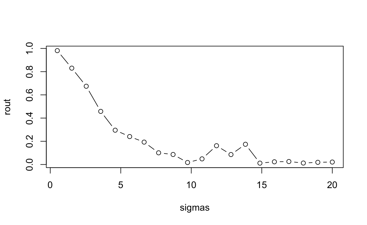
R-squared tanks hard with increasing sigma, even though the model is completely correct in every respect. After addressing that this might not always be the best measure to use, we probably want to consider some alternatives. Other measured that can be used instead of R-squared would include Mean Absolute Error, or Root Mean Squared Error.
This information is from https://data.library.virginia.edu/is-r-squared-useless/.