In this project, I use gradient tree boosting to predict how often someone will be absent from work. The data set is from UC Irvine’s Machine Learning Repository. The data uses records ranging from 2007-2010 from a Brazilian company. There are 740 observations with 21 different attributes.
As you can see below, the data set proves to be fairly clean. There are not noticeable outliers, and the observations all seem to be reasonable.
psych::describe(Absenteeism_at_work)
                                vars   n      mean       sd median
ID                                 1 740     18.02    11.02     18
Reason for absence                 2 740     19.22     8.43     23
Month of absence                   3 740      6.32     3.44      6
Day of the week                    4 740      3.91     1.42      4
Seasons                            5 740      2.54     1.11      3
Transportation expense             6 740    221.33    66.95    225
Distance from Residence to Work    7 740     29.63    14.84     26
Service time                       8 740     12.55     4.38     13
Age                                9 740     36.45     6.48     37
Work load Average/day             10 740 271490.24 39058.12 264249
Hit target                        11 740     94.59     3.78     95
Disciplinary failure              12 740      0.05     0.23      0
Education                         13 740      1.29     0.67      1
Son                               14 740      1.02     1.10      1
Social drinker                    15 740      0.57     0.50      1
Social smoker                     16 740      0.07     0.26      0
Pet                               17 740      0.75     1.32      0
Weight                            18 740     79.04    12.88     83
Height                            19 740    172.11     6.03    170
Body mass index                   20 740     26.68     4.29     25
Absenteeism time in hours         21 740      6.92    13.33      3
                                  trimmed      mad    min    max
ID                                  17.87    14.83      1     36
Reason for absence                  20.36     7.41      0     28
Month of absence                     6.29     4.45      0     12
Day of the week                      3.89     1.48      2      6
Seasons                              2.56     1.48      1      4
Transportation expense             217.93    68.20    118    388
Distance from Residence to Work     29.40    16.31      5     52
Service time                        12.76     5.93      1     29
Age                                 35.83     5.93     27     58
Work load Average/day           267438.64 30547.49 205917 378884
Hit target                          95.01     2.97     81    100
Disciplinary failure                 0.00     0.00      0      1
Education                            1.11     0.00      1      4
Son                                  0.86     1.48      0      4
Social drinker                       0.58     0.00      0      1
Social smoker                        0.00     0.00      0      1
Pet                                  0.46     0.00      0      8
Weight                              78.99    16.31     56    108
Height                             171.02     2.97    163    196
Body mass index                     26.65     4.45     19     38
Absenteeism time in hours            4.33     2.97      0    120
                                 range  skew kurtosis      se
ID                                  35  0.02    -1.26    0.41
Reason for absence                  28 -0.91    -0.27    0.31
Month of absence                    12  0.07    -1.26    0.13
Day of the week                      4  0.10    -1.29    0.05
Seasons                              3 -0.04    -1.35    0.04
Transportation expense             270  0.39    -0.33    2.46
Distance from Residence to Work     47  0.31    -1.27    0.55
Service time                        28  0.00     0.66    0.16
Age                                 31  0.69     0.41    0.24
Work load Average/day           172967  0.96     0.60 1435.80
Hit target                          19 -1.26     2.38    0.14
Disciplinary failure                 1  3.94    13.51    0.01
Education                            3  2.10     2.94    0.02
Son                                  4  1.08     0.73    0.04
Social drinker                       1 -0.27    -1.93    0.02
Social smoker                        1  3.28     8.75    0.01
Pet                                  8  2.72     9.57    0.05
Weight                              52  0.02    -0.92    0.47
Height                              33  2.56     7.23    0.22
Body mass index                     19  0.30    -0.33    0.16
Absenteeism time in hours          120  5.70    38.40    0.49
Decision trees are a simple machine learning algorithm that are relatively easy to understand and employ. However, they often overfit the data, making the models less accurate when the testing data is used. To prevent this overfitting, there are models that combine multiple trees, increasing accuracy. In this project, I use gradient tree boosting to accomplish this. Boosting means combining many connected weak learners to make a strong learner. Each tree tries to minimize the errors of the previous tree. In boosting, trees are weak learners, but adding many of them in sequence and focusing on the errors from the previous tree makes them very efficient and accurate. Because trees are added sequentially, this algorithm learns more slowly, meaning it will perform better. Gradient boosting sequentially combines the weak learners so the new learner fits to the errors of the previous tree. The final model then aggregates these steps, making a strong learner.
set.seed(45678)
trainIndex <- createDataPartition(Absenteeism_at_work$`Absenteeism time in hours`, p = .6, list = FALSE, times = 1)
AbsentTrain <- Absenteeism_at_work[ trainIndex,]
AbsentTest  <- Absenteeism_at_work[-trainIndex,]
set.seed(7777)
absentgbm<- train(
  form = `Absenteeism time in hours` ~ factor(`Month of absence`)+factor(`Day of the week`)+factor(Seasons)+factor(`Reason for absence`)+factor(`Disciplinary failure`)+factor(Education)+factor(`Social drinker`)+factor(`Social smoker`)+`Transportation expense`+`Distance from Residence to Work`+`Service time`+Age+`Work load Average/day`+`Hit target`+Son+Pet+Weight+Height+`Body mass index`,
  data = AbsentTrain,
  trControl = trainControl(method = "cv", number = 10),
  method = "gbm",
  tuneLength = 10,
  verbose=FALSE)

#summary(absentgbm)

#had to add something
library(gbm)
V<-caret::varImp(absentgbm, n.trees=500)$importance%>%
  arrange(desc(Overall))

knitr::kable(V)%>%
  kableExtra::kable_styling("striped")%>%
  kableExtra::scroll_box(width = "50%",height="300px")
| Overall | |
|---|---|
| Age | 100.0000000 |
| Height | 90.1503788 |
Work load Average/day
|
88.0872168 |
Hit target
|
84.4842211 |
factor(Reason for absence)19
|
52.7179654 |
Transportation expense
|
47.4386602 |
factor(Reason for absence)13
|
45.5583793 |
| Pet | 43.8779913 |
Distance from Residence to Work
|
40.8980337 |
| Son | 37.2103543 |
| Weight | 36.9874263 |
factor(Reason for absence)11
|
19.4297497 |
factor(Month of absence)3
|
17.4780818 |
factor(Month of absence)4
|
15.1799026 |
| factor(Seasons)4 | 12.3049202 |
factor(Month of absence)11
|
11.8735890 |
Service time
|
11.4098887 |
Body mass index
|
10.5634012 |
factor(Month of absence)7
|
10.4736503 |
| factor(Seasons)3 | 8.3468553 |
factor(Month of absence)12
|
7.3945781 |
factor(Day of the week)3
|
7.2818424 |
factor(Reason for absence)23
|
6.1882563 |
factor(Day of the week)4
|
6.0842947 |
factor(Disciplinary failure)1
|
5.8735298 |
factor(Reason for absence)28
|
5.3082485 |
factor(Social drinker)1
|
4.0625461 |
| factor(Seasons)2 | 3.2029279 |
factor(Reason for absence)14
|
1.1231799 |
factor(Reason for absence)27
|
1.0241352 |
factor(Reason for absence)22
|
1.0169829 |
factor(Social smoker)1
|
0.9510118 |
factor(Reason for absence)10
|
0.9013602 |
factor(Month of absence)6
|
0.8385516 |
factor(Day of the week)6
|
0.5774088 |
| factor(Education)3 | 0.5706620 |
factor(Month of absence)2
|
0.4883797 |
factor(Month of absence)10
|
0.4721127 |
factor(Reason for absence)26
|
0.3045717 |
factor(Month of absence)1
|
0.2535103 |
factor(Month of absence)5
|
0.0000000 |
factor(Month of absence)8
|
0.0000000 |
factor(Month of absence)9
|
0.0000000 |
factor(Day of the week)5
|
0.0000000 |
factor(Reason for absence)1
|
0.0000000 |
factor(Reason for absence)2
|
0.0000000 |
factor(Reason for absence)3
|
0.0000000 |
factor(Reason for absence)4
|
0.0000000 |
factor(Reason for absence)5
|
0.0000000 |
factor(Reason for absence)6
|
0.0000000 |
factor(Reason for absence)7
|
0.0000000 |
factor(Reason for absence)8
|
0.0000000 |
factor(Reason for absence)9
|
0.0000000 |
factor(Reason for absence)12
|
0.0000000 |
factor(Reason for absence)15
|
0.0000000 |
factor(Reason for absence)16
|
0.0000000 |
factor(Reason for absence)18
|
0.0000000 |
factor(Reason for absence)21
|
0.0000000 |
factor(Reason for absence)24
|
0.0000000 |
factor(Reason for absence)25
|
0.0000000 |
| factor(Education)2 | 0.0000000 |
| factor(Education)4 | 0.0000000 |
ggplot2::ggplot(V, aes(x=reorder(rownames(V),Overall), y=Overall)) +
geom_point( color="blue", size=4, alpha=0.6)+
geom_segment( aes(x=rownames(V), xend=rownames(V), y=0, yend=Overall),
color='skyblue') +
xlab('Variable')+
ylab('Overall Importance')+
theme_light() +
coord_flip()
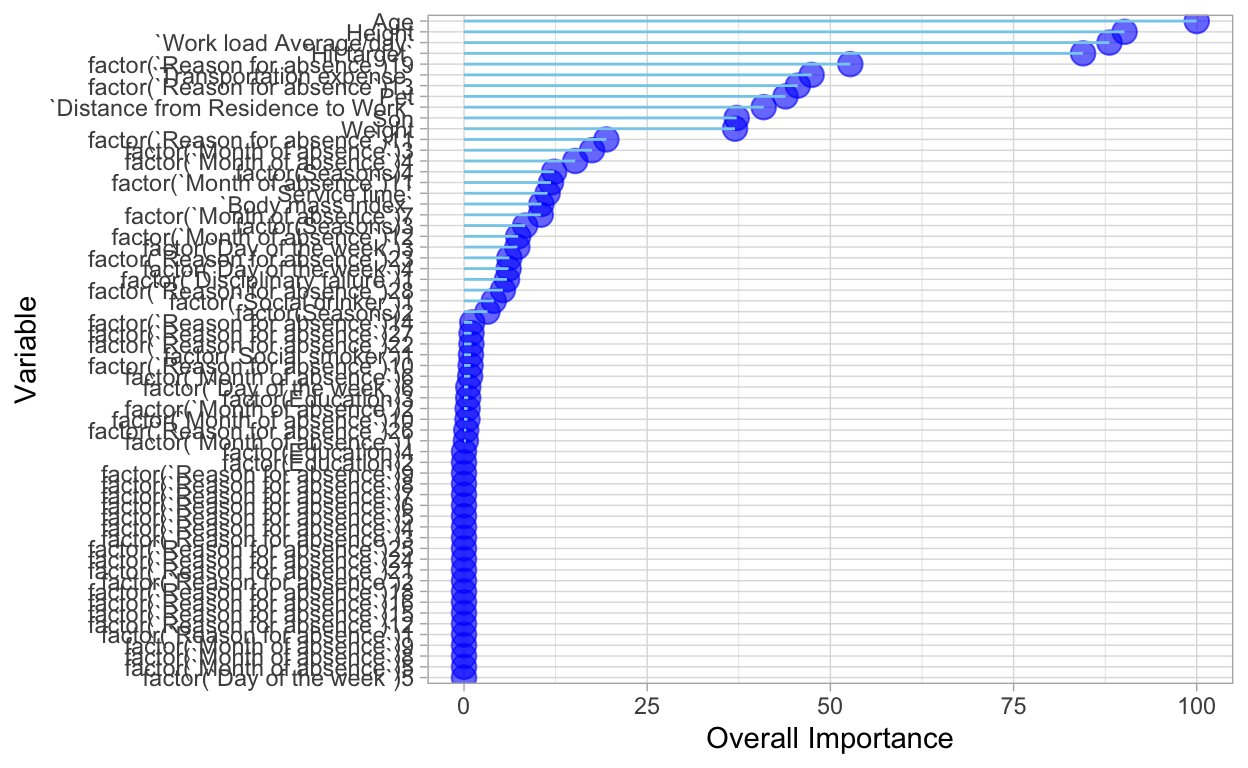
This chart shows the importance of each variable available in the dataset. The higher the importance, the more effect it has on how often one is absent from work.
gridExtra::grid.arrange(
  pdp::partial(absentgbm, pred.var = "Age", plot = TRUE, rug = TRUE,
              plot.engine = "ggplot2"),
  pdp::partial(absentgbm, pred.var = "Height", plot = TRUE, rug = TRUE,
              plot.engine = "ggplot2"),
  ncol = 2
)
pd <- pdp::partial(absentgbm, pred.var = c("Age","Height"))

# Default PDP
pdp::plotPartial(pd)
rwb <- colorRampPalette(c("darkred", "white", "pink"))
pdp::plotPartial(pd, contour = TRUE, col.regions = rwb)
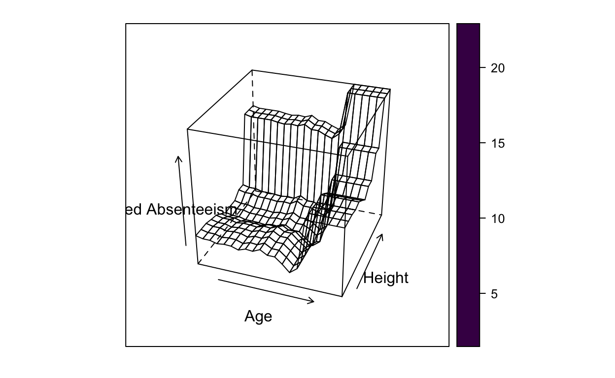
pdp::plotPartial(pd, levelplot = FALSE, zlab = "Predicted Absenteeism", colorkey = TRUE,
                    screen = list(z = -20, x = -60))
dens <- akima::interp(x = pd$Age, y = pd$`Height`, z = pd$yhat)

# 3D partial dependence plot with a coloring scale
p3 <- plotly::plot_ly(x = dens$x,
          y = dens$y,
          z = dens$z,
          colors = c("blue", "grey", "red"),
          type = "surface")
# Add axis labels for 3D plots

p3 <- p3%>% plotly::layout(scene = list(xaxis = list(title = 'Age'),
                     yaxis = list(title = 'Height'),
                     zaxis = list(title = 'Predicted Absence')))
p3
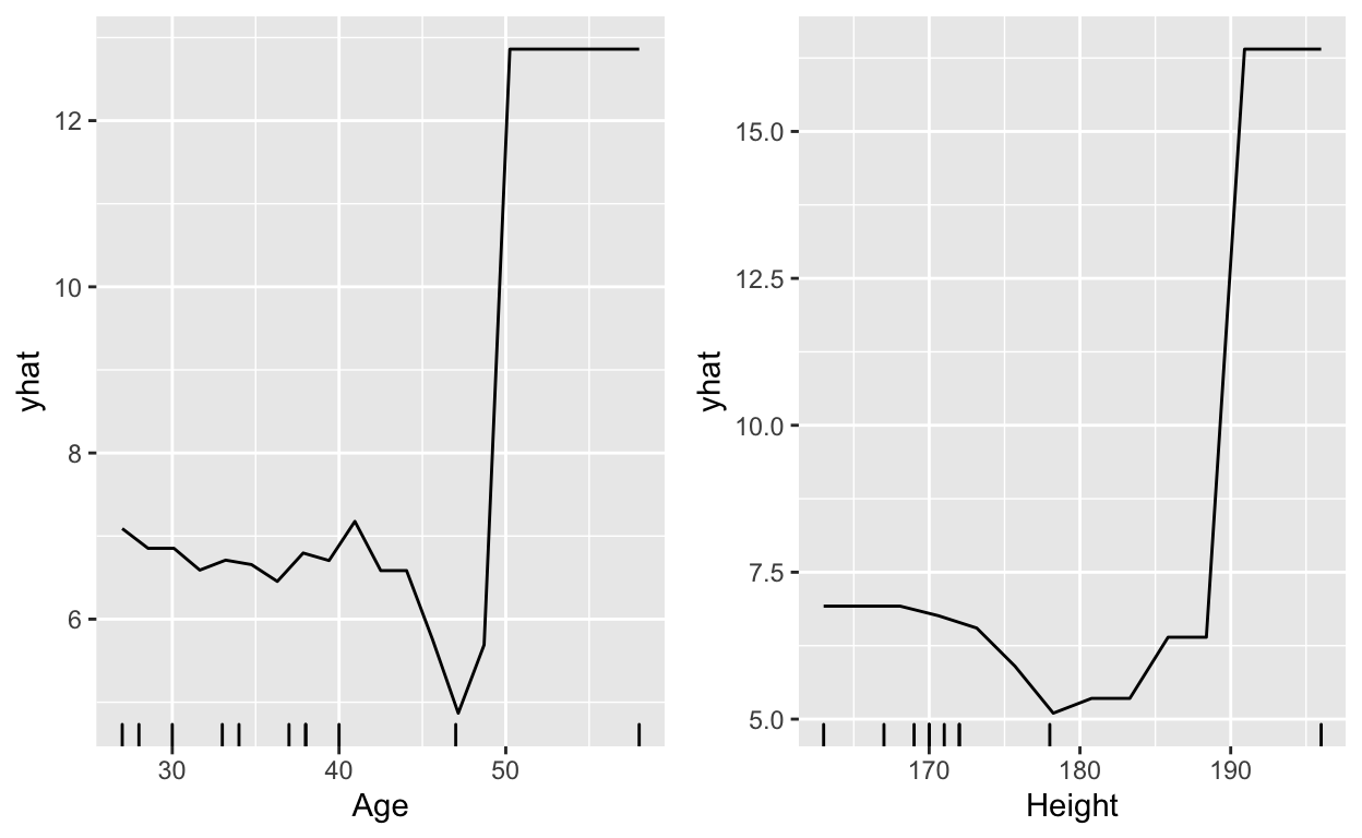
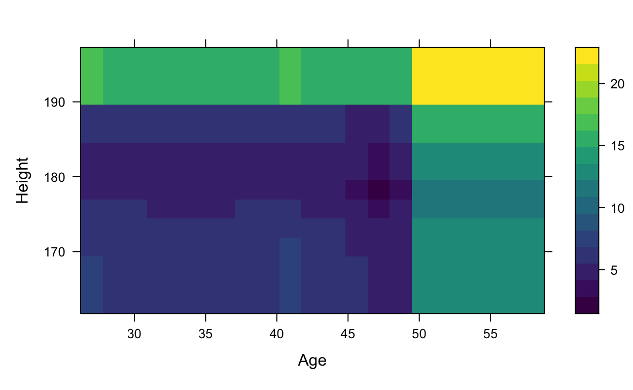
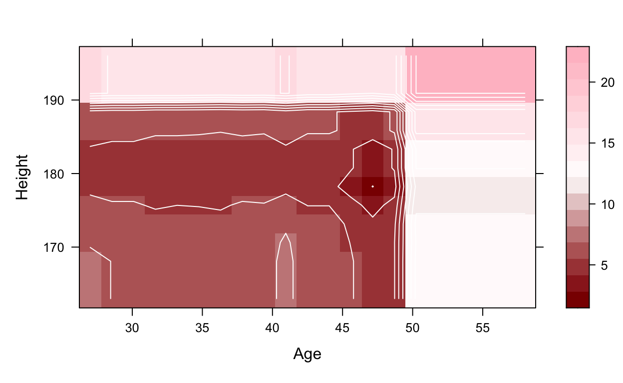
As you can see from these previous graphs and visualizations, age and height both have an effect on being absent from work. In general, the older someone is and the taller someone is, the more likely they are to miss work. However, it is an unsound conclusion to say that the taller you are, the more you miss work. Because this data set does not include a variable for sex, we can assume from the results that males will miss work more, assuming they are taller on average.
These results could be useful in various situations. I would say it could be beneficial in the hiring process to be able to identify those who will be more likely to be absent, as most employers do not want to hire someone that will be absent a large amount of time. Although we only used Age and Height in this example, other variables did have an effect on the predictions and could be used in other ways as well. For example, it might be beneficial to use the Average work load to see what the optimal amount is to reduce absenteeism.